School of Electrical and Computer Engineering Georgia Institute of Technology
Broadband Wireless Networking Lab

ECE 8863: Cognitive Radio Networks
Lab 2: Spectrum Sensing
Spectrum sensing is one of the fundamental functionalities of cognitive radio that assures the protection of primary user communications from harmful interference. The speed and accuracy of spectrum sensing techniques are essential factors in the performance of cognitive radio networks. The limitations imposed by computational complexity and a shortened monitoring time impede the success of spectrum sensing operation performed by cognitive radio nodes.
In this lab, we aim to design and implement an energy detector and measure its performance on the CR testbed. After finishing this lab, you will know how to
Environment Setup
Log into your account on host laptops 1 & 2.
Create a directory: lab2. This is your work area: <lab2>.
Download the following files to <lab2>. Files: lab2_energy_detector.grc, lab2_energy_detector_sweep.py, lab2_PU_Transmitter.grc, lab2_PU_dynamic.py.
Lab Procedures
In this lab, we are going to develop an energy detector to perform spectrum sensing for cognitive radio transceivers. The energy detection is performed in the frequency domain. Figure 1 shows a block diagram of the energy detector that you are going to develop.
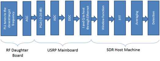
Figure 1: Block Diagram of Energy Detector Implementation Using USRP
In this lab, we are going to develop the code that runs at the SDR host machine section. The detector development will be conducted in three stages. Figure 2 shows the setup for the second lab.
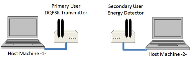
Figure 2. Lab 2 Setup
In the first stage, we setup the primary user transmission in Host 1. In the second stage, we develop the energy detector on GRC environment and then using Python environment to detect Primary user transmissions. Third, we develop an automatic spectrum sensing scanner to detect unknown transmission on a given spectrum range.
Table 1: Summary of CR Sensing Specifications.
Parameter |
Value |
| Sensing bandwidth | 200 kHz |
| Sample rate | 200 kSPS |
| AGC | 0 dB |
| FFT Size | 1024 |
| Windowing function | Blackman-Harris |
| Averaging Size | 10 |
| Probability of false alarm | 0.1 |
| Probability of detection | 0.9 |
| Scanning range | 899-901 MHz |
| PU USRP | 192.168.40.1 |
| SU USRP | 192.168.40.3 |
A. PU Transmission Setup
Start with Host 1. Open lab2_PU_Transmitter.grc file. This is a simple DQPSK transmitter with a simple spectrum analyzer at the receiving side to verify the transmission.
Make sure that the parameters are set as per Table 1. Use antenna VERT900.
Generate and execute the flow graph.
Verify the transmission through the FFT plot.
Task 1: Estimate and record the maximum received power level (in dBm) from the spectrum plot at the receiver.
B. Energy Detector and Calibration
Task 2: Observe the activities in the spectrum band through the FFT plot and record what you see.
Task 3: Estimate received power at the receiver and record the value in dBm.
Task 4: Calculate the path loss in indoor environment using the estimated values obtained from Task 1 and Task 3. For simplicity, you can assume the power calculated in Task1 as the transmission power.
Hw1 Q4:
- In Task 2, do you observe any activity in the spectrum? If yes, what are these activities (recall that Host 1 is not transmitting)? If no, what do you see in the spectrum? What is the level of noise floor in dBm?
- Calculate the path loss using the ITU indoor path loss model given in the Appendix, and compare the result to the one obtained in Task 4. Do they match? Tell us why if they don't match.
C. Spectrum Sensing using Energy Detector:
Task 5: Change the default settings of the options to make the scanning more effective.
Task 6: See if the energy detector can detect the PU transmission at the frequency you specified.
Task 7: See if the energy detector can effectively detect the PU transmission.
Hw1 Q5:
- How do you set the threshold for the detection in Task 5?
- Which options or settings did you change to improve the speed of the detection in Task 5?
- Can the energy detector detect the PU transmission in Task 6? If yes, explain the PU activity behavior and list your your energy detector settings to show that the detection is effective. If no, tell us why the detection is not possible.
- Repeat the previous question for the case in Task 7.
Show your results to a TA. This is the only check point.
The ITU indoor path loss model is formally expressed as:
![]()
where
L = the total path loss. Unit: decibel (dB).
f = Frequency of transmission. Unit: megahertz(MHz).
d = Distance. Unit: meter (m).
N = The distance power loss coefficient.
n = Number of floors between the transmitter and receiver.
Pf(n) = the floor loss penetration factor.
The distance power loss coefficient, N is the quantity that expresses the loss of signal power with distance. This coefficient is an empirical one. Some values are provided in Table 2.
Table 2. Distance Power Loss Coefficient
Frequency Band |
Residential Area |
Office Area |
Commercial Area |
900 MHz |
N/A |
33 |
20 |
The floor penetration loss factor is an empirical constant dependent on the number of floors the waves need to penetrate. Some values are tabulated in Table 3.
Table 3. Floor Penetration Loss Factor
Frequency Band |
Number of Floors |
Residential Area |
Office Area |
Commercial Area |
900 MHz |
1 |
N/A |
9 |
N/A |
900 MHz |
2 |
N/A |
19 |
N/A |
900 MHz |
3 |
N/A |
24 |
N/A |
Questions? E-mail: infocom@ece.gatech.edu
You are visitor:
since 04/22/1997.